Case Study: Police Stops in Oakland

For this EDA, we’ll work with data on police stops in Oakland, California, that have been pre-cleaned and released by the Stanford Open Policing Project (Pierson et al. 2020).
We’ll be following the checklist from Peng and Matsui (2016).
We’ll also be learning to use the skimr and visdat packages

Peng and Matsui (2016)

Formulate your question
Read in your data
Check the packaging
Look at the top and the bottom of your data
Check your “n”s
Validate with at least one external data source
Make a plot
Try the easy solution first
Follow up

1. Formulate your question

The Black Lives Matter protests over the last several years have made us aware of the racial aspects of policing.
Here we’re specifically interested in
1. Whether Black people in Oakland might be more likely to be stopped than White people
2. Whether Black people who are stopped might be more likely to have contraband
These aren’t very precise, but that’s okay: Part of the goal of EDA is to clarify and refine our research questions

Set up our workspace

Dedicated project folder
Optional: Create an RStudio Project
Clean R session
More on project management and organization later in the semester

Packages

library(tidyverse)   # for working with the data
library(lubridate)   # for working with datetime data

library(skimr)       # generate a text-based overview of the data
library(visdat)      # generate plots visualizing data types and missingness
library(plotly)      # quickly create interactive plots

Get the Data

We’ll be using data on police stops in Oakland, California, collected and published by the Stanford Open Policing Project.
For reproducibility, we’ll write a bit of code that automatically downloads the data
To get the download URL:
1. https://openpolicing.stanford.edu/data/
2. Scroll down to Oakland
3. Right-click on the file symbol to copy the URL
README: https://github.com/stanford-policylab/opp/blob/master/data_readme.md.

data_dir = 'data'
target_file = file.path(data_dir, 'oakland.zip')

if (!dir.exists(data_dir)) {
    dir.create(data_dir)
}
if (!file.exists(target_file)) {
    download.file('https://stacks.stanford.edu/file/druid:yg821jf8611/yg821jf8611_ca_oakland_2020_04_01.csv.zip', 
                  target_file)
}

2. Read in your data

The dataset is a zipped csv or comma-separated value file. CSVs are structured like Excel spreadsheets, but are stored in plain text rather than Excel’s format.

dataf = read_csv(target_file)

Rows: 133407 Columns: 28
── Column specification ────────────────────────────────────────────────────────────────────────────
Delimiter: ","
chr  (16): raw_row_number, location, beat, subject_race, subject_sex, officer_assignment, type, ...
dbl   (3): lat, lng, subject_age
lgl   (7): arrest_made, citation_issued, warning_issued, contraband_found, contraband_drugs, con...
date  (1): date
time  (1): time

ℹ Use `spec()` to retrieve the full column specification for this data.
ℹ Specify the column types or set `show_col_types = FALSE` to quiet this message.

3. Check the packaging

Peng and Matsui (2016) use some base R functions to look at dimensions of the dataframe and column (variable) types. skimr is more powerful.

## May take a couple of seconds
skim(dataf)

── Data Summary ────────────────────────
                           Values
Name                       dataf 
Number of rows             133407
Number of columns          28    
_______________________          
Column type frequency:           
  character                16    
  Date                     1     
  difftime                 1     
  logical                  7     
  numeric                  3     
________________________         
Group variables            None  

── Variable type: character ────────────────────────────────────────────────────────────────────────
   skim_variable                 n_missing complete_rate min max empty n_unique whitespace
 1 raw_row_number                        0        1        1  71     0   133407          0
 2 location                             51        1.00     1  78     0    60723          0
 3 beat                              72424        0.457    3  19     0      129          0
 4 subject_race                          0        1        5  22     0        5          0
 5 subject_sex                          90        0.999    4   6     0        2          0
 6 officer_assignment               121431        0.0898   5  97     0       20          0
 7 type                              20066        0.850    9  10     0        2          0
 8 outcome                           34107        0.744    6   8     0        3          0
 9 search_basis                      92250        0.309    5  14     0        3          0
10 reason_for_stop                       0        1       14 197     0      113          0
11 use_of_force_description         116734        0.125   10  10     0        1          0
12 raw_subject_sdrace                    0        1        1   1     0        7          0
13 raw_subject_resultofencounter         0        1        7 213     0      315          0
14 raw_subject_searchconducted           0        1        2  24     0       34          0
15 raw_subject_typeofsearch          52186        0.609    2 112     0      417          0
16 raw_subject_resultofsearch       111633        0.163    5  95     0      298          0

── Variable type: Date ─────────────────────────────────────────────────────────────────────────────
  skim_variable n_missing complete_rate min        max        median     n_unique
1 date                  2          1.00 2013-04-01 2017-12-31 2015-07-19     1638

── Variable type: difftime ─────────────────────────────────────────────────────────────────────────
  skim_variable n_missing complete_rate min    max        median n_unique
1 time                  2          1.00 0 secs 86340 secs 16:12      1439

── Variable type: logical ──────────────────────────────────────────────────────────────────────────
  skim_variable      n_missing complete_rate   mean count                  
1 arrest_made                0         1     0.121  FAL: 117217, TRU: 16190
2 citation_issued            0         1     0.394  FAL: 80836, TRU: 52571 
3 warning_issued             0         1     0.231  FAL: 102545, TRU: 30862
4 contraband_found       92250         0.309 0.149  FAL: 35005, TRU: 6152  
5 contraband_drugs       92250         0.309 0.0844 FAL: 37684, TRU: 3473  
6 contraband_weapons     92250         0.309 0.0299 FAL: 39928, TRU: 1229  
7 search_conducted           0         1     0.309  FAL: 92250, TRU: 41157 

── Variable type: numeric ──────────────────────────────────────────────────────────────────────────
  skim_variable n_missing complete_rate   mean      sd     p0    p25    p50    p75   p100 hist 
1 lat                 114         0.999   37.8  0.0284   37.4   37.8   37.8   37.8   38.1 ▁▁▇▁▁
2 lng                 114         0.999 -122.   0.0432 -122.  -122.  -122.  -122.  -119.  ▇▁▁▁▁
3 subject_age      102724         0.230   33.2 13.3      10     23     29     41     97   ▇▆▃▁▁

How many rows and columns?
What variables are represented as different variable types?
Are there any types that might indicate parsing problems?

133k rows (observations); 28 columns (variables)
16 variables are handled as characters
- raw_row_number has 1 unique value per row
  - So it’s probably some kind of identifier
- subject_race and subject_sex have just 5 and 2 unique values
  - These are probably categorical variables represented as characters
- Similarly with type, outcome, and search_basis
  - Though these have lots of missing values (high n_missing, low complete_rate)
1 variable represents the date, and another is difftime
- ?difftime tells us that difftime is used to represent intervals or “time differences”
7 logical variables
- A lot of these look like coded outcomes that we might be interested in, eg, search_conducted and contraband_found
- search_conducted has no missing values, but contraband_found has a lot of missing values

For our motivating questions

Good: subject_race is 100% complete
Also good: search_conducted is also 100% complete
Potentially worrisome: contraband_found is only 31% complete

Missing values

Let’s use visdat::vis_miss()to
- visualize missing values and
- check what’s up with contraband_found.

But this raises an error about large data

vis_miss(dataf)

Error in `test_if_large_data()`:
! Data exceeds recommended size for visualisation
Consider downsampling your data with `dplyr::slice_sample()`
Or set argument, `warn_large_data` = `FALSE`

So we’ll use sample_n() to draw a subset

set.seed(2021-09-28)
dataf_smol = sample_n(dataf, 1000)

vis_miss(dataf_smol)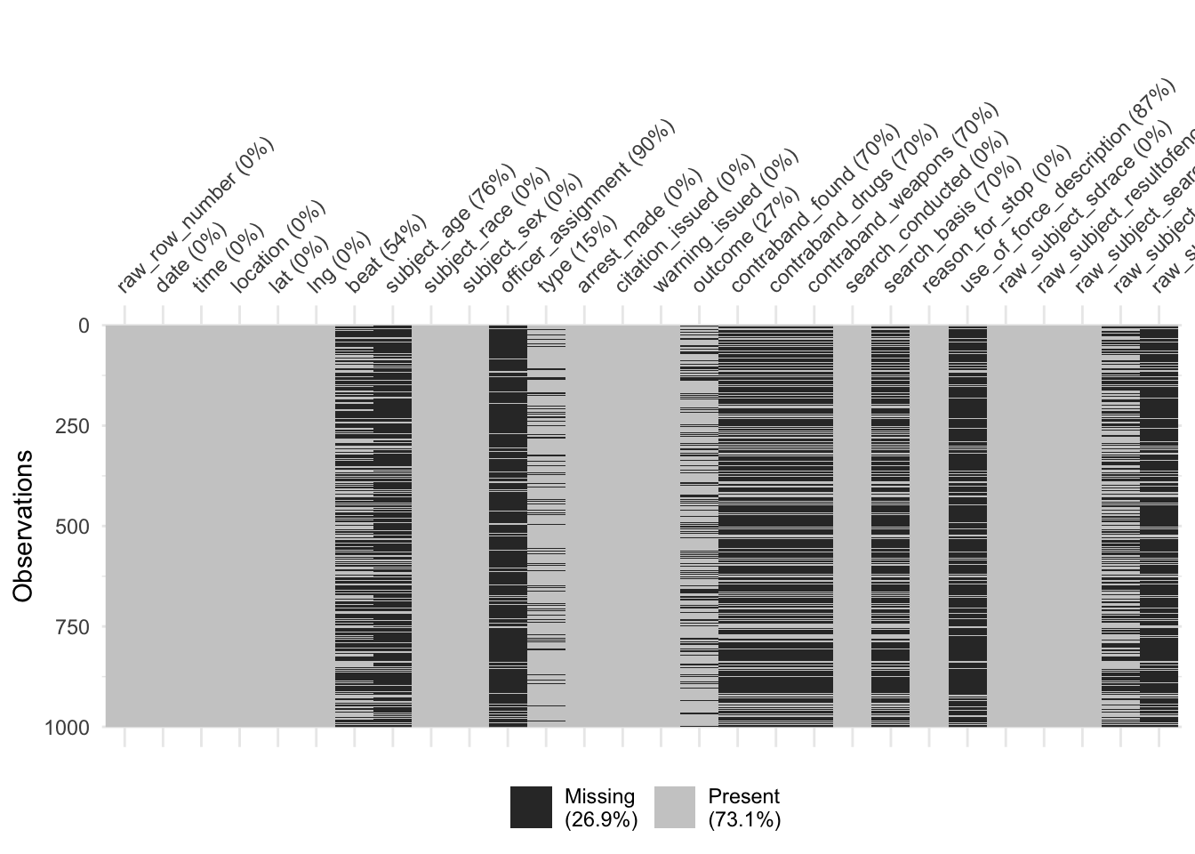

Arguments in vis_miss() are useful for picking up patterns in missing values

## cluster = TRUE uses hierarchical clustering to order the rows
vis_miss(dataf_smol, cluster = TRUE) +
    coord_flip()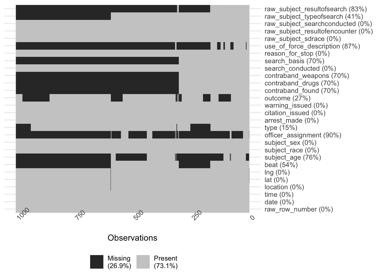

Several variables related to search outcomes are missing together

contraband_found, contraband_drugs, contraband_weapons, search_basis, use_of_force_description, raw_subject_typeofsearch, and raw_subject_resultofsearch

However, search_conducted is complete

A critical question

When a search has been conducted, do we know whether contraband was found?

Or: are there cases where a search was conducted, but contraband_found is missing?

dataf  |>  
    filter(search_conducted) |>
    count(search_conducted, is.na(contraband_found))

# A tibble: 1 × 3
  search_conducted `is.na(contraband_found)`     n
  <lgl>            <lgl>                     <int>
1 TRUE             FALSE                     41157

4. Look at the top and the bottom of your data

With 28 columns, the dataframe is too wide to print in a readable way.
Instead we’ll use the base R function View() in an interactive session
- An Excel-like spreadsheet presentation
View() can cause significant problems if you use it with a large dataframe on a slower machine
- We’ll use a pipe:
  - First extract the head() or tail() of the dataset
  - Then View() it
- We’ll also use dataf_smol

if (interactive()) {
    dataf |> 
        head() |> 
        View()
    
    dataf |> 
        tail() |> 
        View()
    
    View(dataf_smol)
}

This is interactive code
- Don’t want it to run when we run the script automatically or render it to HTML
- Use if with interactive() or rlang::is_interactive()

Some of my observations:

The ID variable raw_row_number can’t be turned into a numeric value
location is a mix of addresses and intersections (“Bond St @ 48TH AVE”)
- If we were going to generate a map using this column, geocoding might be tricky
- Fortunately we also get latitude and longitude columns
use_of_force_description doesn’t seem to be a descriptive text field; instead it seems to be mostly missing or “handcuffed”

We can also use skimr to check data quality by looking at the minimum and maximum values. Do these ranges make sense for what we expect the variable to be?

skim(dataf)

── Data Summary ────────────────────────
                           Values
Name                       dataf 
Number of rows             133407
Number of columns          28    
_______________________          
Column type frequency:           
  character                16    
  Date                     1     
  difftime                 1     
  logical                  7     
  numeric                  3     
________________________         
Group variables            None  

── Variable type: character ────────────────────────────────────────────────────────────────────────
   skim_variable                 n_missing complete_rate min max empty n_unique whitespace
 1 raw_row_number                        0        1        1  71     0   133407          0
 2 location                             51        1.00     1  78     0    60723          0
 3 beat                              72424        0.457    3  19     0      129          0
 4 subject_race                          0        1        5  22     0        5          0
 5 subject_sex                          90        0.999    4   6     0        2          0
 6 officer_assignment               121431        0.0898   5  97     0       20          0
 7 type                              20066        0.850    9  10     0        2          0
 8 outcome                           34107        0.744    6   8     0        3          0
 9 search_basis                      92250        0.309    5  14     0        3          0
10 reason_for_stop                       0        1       14 197     0      113          0
11 use_of_force_description         116734        0.125   10  10     0        1          0
12 raw_subject_sdrace                    0        1        1   1     0        7          0
13 raw_subject_resultofencounter         0        1        7 213     0      315          0
14 raw_subject_searchconducted           0        1        2  24     0       34          0
15 raw_subject_typeofsearch          52186        0.609    2 112     0      417          0
16 raw_subject_resultofsearch       111633        0.163    5  95     0      298          0

── Variable type: Date ─────────────────────────────────────────────────────────────────────────────
  skim_variable n_missing complete_rate min        max        median     n_unique
1 date                  2          1.00 2013-04-01 2017-12-31 2015-07-19     1638

── Variable type: difftime ─────────────────────────────────────────────────────────────────────────
  skim_variable n_missing complete_rate min    max        median n_unique
1 time                  2          1.00 0 secs 86340 secs 16:12      1439

── Variable type: logical ──────────────────────────────────────────────────────────────────────────
  skim_variable      n_missing complete_rate   mean count                  
1 arrest_made                0         1     0.121  FAL: 117217, TRU: 16190
2 citation_issued            0         1     0.394  FAL: 80836, TRU: 52571 
3 warning_issued             0         1     0.231  FAL: 102545, TRU: 30862
4 contraband_found       92250         0.309 0.149  FAL: 35005, TRU: 6152  
5 contraband_drugs       92250         0.309 0.0844 FAL: 37684, TRU: 3473  
6 contraband_weapons     92250         0.309 0.0299 FAL: 39928, TRU: 1229  
7 search_conducted           0         1     0.309  FAL: 92250, TRU: 41157 

── Variable type: numeric ──────────────────────────────────────────────────────────────────────────
  skim_variable n_missing complete_rate   mean      sd     p0    p25    p50    p75   p100 hist 
1 lat                 114         0.999   37.8  0.0284   37.4   37.8   37.8   37.8   38.1 ▁▁▇▁▁
2 lng                 114         0.999 -122.   0.0432 -122.  -122.  -122.  -122.  -119.  ▇▁▁▁▁
3 subject_age      102724         0.230   33.2 13.3      10     23     29     41     97   ▇▆▃▁▁

More observations:

Date range is April 1, 2013 to December 31, 2017
- If we break things down by year, we should expect 2013 to have fewer cases
- For some purposes, we might need to exclude 2013 data
  filter(dataf, date >= '2014-01-01')
Age range is from 10 years old (!) to 97 (!)
- Median (p50) is 29; 50% of values are between 23 and 41
- For some purposes, we might need to restrict the analysis to working-age adults
  filter(dataf, subject_age >= 18, subject_age < 65)

5. Check your Ns (and) 6. Validate with at least one external data source

Peng and Matsui (2016) use an air quality example with a regular sampling rate
- so they can calculate exactly how many observations they should have
We can’t do that here
- So we’ll combine steps 5 and 6 together

A web search leads us to this City of Oakland page on police stop data: https://www.oaklandca.gov/resources/stop-data
- The page mentions a Stanford study that was released in June 2016
- Recall we got our data from the Stanford Open Policing Project
- Our data run April 2013 through December 2017
- So there’s a good chance we’re using a superset of the “Stanford study” data
- Though the links under that section don’t have nice descriptive tables

Let’s try Historical Stop Data and Reports
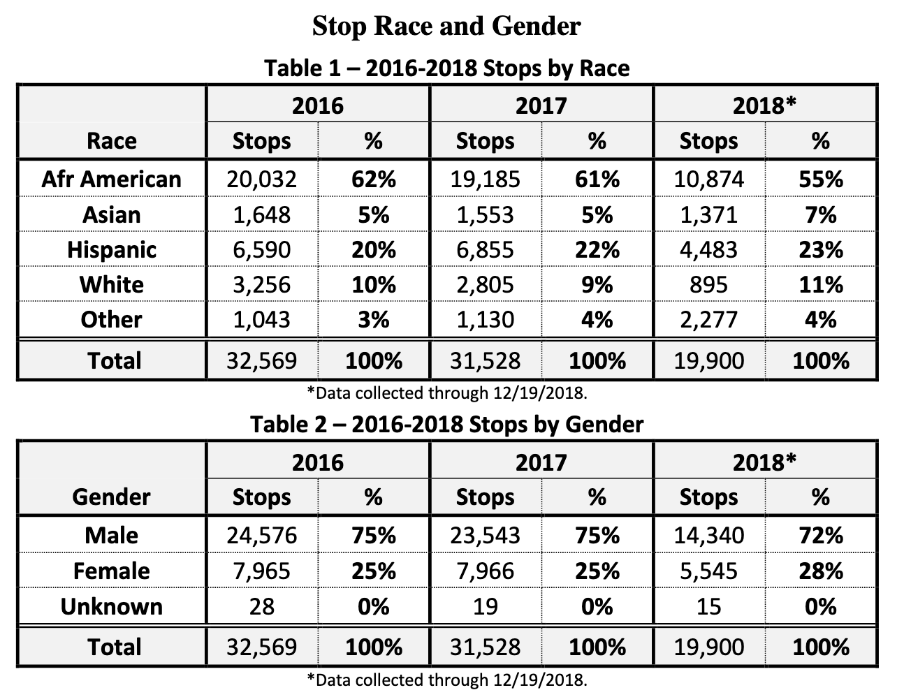
Then OPD Racial Impact Report: 2016-2018
- Page 8 has two summary tables that we can compare to our data

Screenshot of the two summary tables from the Oakland report. Source: https://cao-94612.s3.amazonaws.com/documents/OPD-Racial-Impact-Report-2016-2018-Final-16Apr19.pdf, page 8

From dates to years

Our data has the particular date of each stop
- We need to extract the year of each stop
  - lubridate::year() does exactly this
- Filter to the years in our data that overlap with the tables
- And then aggregate by year and gender using count

dataf |> 
    mutate(year = year(date)) |> 
    filter(year %in% c(2016, 2017)) |> 
    count(year)

# A tibble: 2 × 2
   year     n
  <dbl> <int>
1  2016 30268
2  2017 30715

dataf |> 
    mutate(year = year(date)) |> 
    filter(year %in% c(2016, 2017)) |> 
    count(year, subject_sex)

# A tibble: 6 × 3
   year subject_sex     n
  <dbl> <chr>       <int>
1  2016 female       7677
2  2016 male        22563
3  2016 <NA>           28
4  2017 female       7879
5  2017 male        22818
6  2017 <NA>           18

For both years, we have fewer observations than the report table indicates
- Could our data have been pre-filtered?
- Let’s check the documentation for our data: https://github.com/stanford-policylab/opp/blob/master/data_readme.md#oakland-ca

“Data is deduplicated on raw columns contactdate, contacttime, streetname, subject_sdrace, subject_sex, and subject_age, reducing the number of records by ~5.2%”

The difference with the report is on this order of magnitude,
But varies within groups by several percentage points
So deduplication might explain the difference
But in a more serious analysis we might want to check, eg, with the Stanford Open Policing folks

## Men in 2016 in the report vs. our data: 8.2%
(24576 - 22563) / 24576

[1] 0.08190918

## Women in 2016 in the report vs. our data: 3.6%
(7965 - 7677) / 7965

[1] 0.03615819

## All of 2016 in the report vs. our data: 7.1%
(32569 - 30268) / 32569

[1] 0.07065

7. Make a plot

Peng and Matsui note that plots are useful for both checking and setting expectations

An expectation we formed earlier: fewer stops in 2013
We can combine pipes with ggplot() to get the year
geom_bar() gives us counts
What’s up with the warnings?

dataf |> 
    mutate(year = year(date)) |> 
    ggplot(aes(year)) +
    geom_bar()

Warning: Removed 2 rows containing non-finite values (`stat_count()`).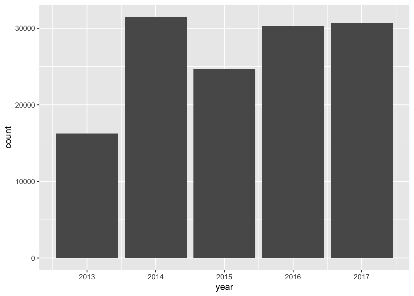

How about counts per year by race/ethnicity?

This version is too hard to read

dataf |> 
    mutate(year = year(date)) |> 
    ggplot(aes(year, fill = subject_race)) +
    geom_bar()

Warning: Removed 2 rows containing non-finite values (`stat_count()`).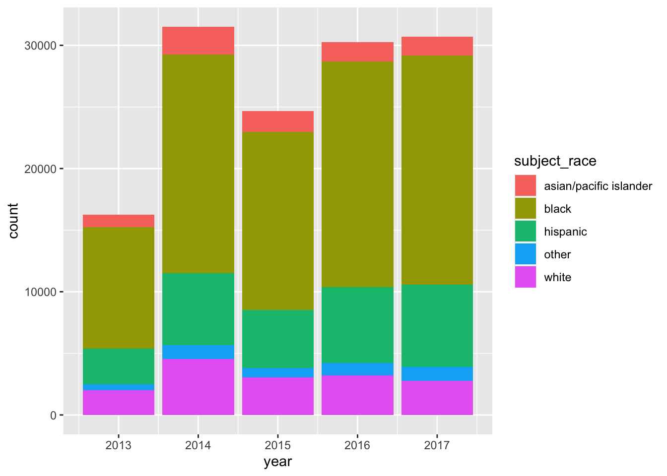

Let’s switch from bars to points and lines and change up the color palette

Why does this produce 2 warnings?

dataf |> 
    mutate(year = year(date)) |> 
    ggplot(aes(year, color = subject_race)) +
    geom_point(stat = 'count') +
    geom_line(stat = 'count') +
    scale_color_brewer(palette = 'Set1')

Warning: Removed 2 rows containing non-finite values (`stat_count()`).
Removed 2 rows containing non-finite values (`stat_count()`).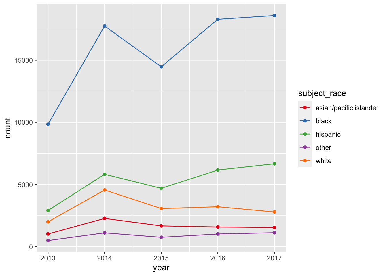

plotly::ggplotly() creates an interactive version of a ggplot object

Why don’t I need to give it the plot we just created?

ggplotly()

Warning: Removed 2 rows containing non-finite values (`stat_count()`).
Removed 2 rows containing non-finite values (`stat_count()`).

These plots confirm our expectation of lower counts in 2013
Do they help us develop any new expectations as we move on to addressing our research questions?

8. Try the easy solution first

Let’s translate our natural-language research questions into statistical questions:

Whether Black people in Oakland might be more likely to be stopped than White people

\[ \Pr(stopped | Black) \textrm{ vs } \Pr(stopped | White) \]

Whether Black people who are stopped might be more likely to have contraband

\[ \Pr(contraband | stopped, searched, Black) \textrm{ vs } \Pr(contraband | stopped, searched, White) \] - The easy solution is to estimate probabilities by calculating rates within groups

Mathematical aside

For Q1, we can’t calculate \(\Pr(stopped | Black)\) directly:
everyone in our data was stopped
But Bayes’ theorem lets us get at the comparison indirectly

\[ \Pr(stopped | Black) = \frac{\Pr(Black | stopped) \times \Pr(stopped)}{\Pr(Black)} \]

\[ \Pr(stopped | Black) : \Pr(stopped | White) = \frac{\Pr(Black|stopped)}{\Pr(Black)} : \frac{\Pr(White|stopped)}{\Pr(White)} \]

\(\Pr(Black)\) is the share of the target population that’s Black
If we assume the target population = residents of Oakland, can use Census data
Why is this assumption probably false? Is it okay to use it anyways?

Stops, by race

\[ \Pr(Black|stopped) \]

dataf |> 
    count(subject_race) |> 
    mutate(share = n / sum(n)) |> 
    arrange(desc(share)) |> 
    mutate(share = scales::percent(share, accuracy = 1))

# A tibble: 5 × 3
  subject_race               n share
  <chr>                  <int> <chr>
1 black                  78925 59%  
2 hispanic               26257 20%  
3 white                  15628 12%  
4 asian/pacific islander  8099 6%   
5 other                   4498 3%

Police stop demographics
- 59% of subjects stopped by police are Black
- 20% are Hispanic
- 12% are White
- 6% are API
Oakland demographics in 2020: https://en.wikipedia.org/wiki/Oakland,_California#Race_and_ethnicity
- 24% of residents are Black
- 27% are Hispanic
- 27% are non-Hispanic White
- 16% are Asian

r/e	residents	stops	ratio
Black	24%	59%	2.5
Hispanic	27%	20%	0.7
White	27%	12%	0.4
API	16%	6%	0.4

Blacks are severely overrepresented in police stops
Hispanics are slightly underrepresented
White and API folks are significantly underrepresented

Searches, by race

What fraction of stops had a search? \[ \Pr(searched | stopped) \]
Are there disparities by race there? \[ \Pr(searched | stopped, Black) \textrm{ vs } \Pr(searched | stopped, White) \]

## What fraction of stops had a search? 
dataf |> 
    count(search_conducted) |> 
    mutate(share = n / sum(n))

# A tibble: 2 × 3
  search_conducted     n share
  <lgl>            <int> <dbl>
1 FALSE            92250 0.691
2 TRUE             41157 0.309

Across all subjects, 31% of stops involved a search.

Now we break down the search rate by race-ethnicity

ggplot(dataf, aes(subject_race, fill = search_conducted)) +
    geom_bar(position = position_fill()) +
    scale_fill_manual(values = c('transparent', 'red'))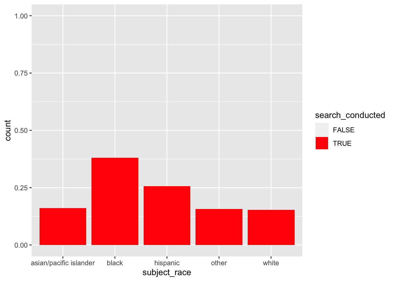

dataf |> 
    count(subject_race, search_conducted) |> 
    group_by(subject_race) |> 
    mutate(rate = n / sum(n)) |> 
    ungroup() |> 
    filter(search_conducted) |> 
    mutate(rate = scales::percent(rate, accuracy = 1))

# A tibble: 5 × 4
  subject_race           search_conducted     n rate 
  <chr>                  <lgl>            <int> <chr>
1 asian/pacific islander TRUE              1304 16%  
2 black                  TRUE             30025 38%  
3 hispanic               TRUE              6722 26%  
4 other                  TRUE               706 16%  
5 white                  TRUE              2400 15%

For all groups, most stops didn’t involve a search
For Black subjects, 38% of stops involved a search
For White subjects, 15% of stops involved a search
Black subjects were about 2.5x more likely to be searched than White subjects

Contraband finds, by race

\[ \Pr(contraband | searched, stopped, Black) \] We want to filter() down to only stops where a search was conducted

dataf |> 
    filter(search_conducted) |> 
    ggplot(aes(subject_race, fill = contraband_found)) +
    geom_bar(position = position_fill()) +
    scale_fill_manual(values = c('transparent', 'blue')) +
    ylim(0, .2)

Warning: Removed 5 rows containing missing values (`geom_bar()`).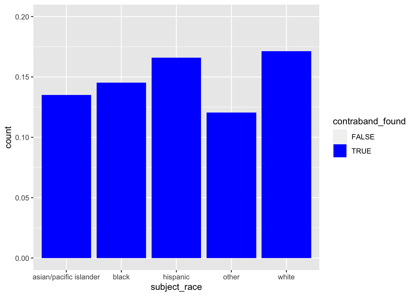

dataf |> 
    filter(search_conducted) |> 
    count(subject_race, contraband_found) |> 
    group_by(subject_race) |> 
    mutate(rate = n / sum(n)) |> 
    ungroup() |> 
    filter(contraband_found) |> 
    mutate(rate = scales::percent(rate, accuracy = 1))

# A tibble: 5 × 4
  subject_race           contraband_found     n rate 
  <chr>                  <lgl>            <int> <chr>
1 asian/pacific islander TRUE               176 13%  
2 black                  TRUE              4364 15%  
3 hispanic               TRUE              1116 17%  
4 other                  TRUE                85 12%  
5 white                  TRUE               411 17%

For Black subjects who were searched, contraband was found 15% of the time
For White subjects, 17% of the time

Results

This preliminary analysis indicates that

Black subjects were more likely to be stopped and searched than White subjects; but,
when they were searched, White subjects were more likely to have contraband.

9. Follow up

What are some further directions we could take this analysis?

Investigate outstanding questions about quality and reliability of the data
- eg, follow up with Stanford Open Policing Project about the difference in row counts
- Fits with epicycle of analysis: checking expectations
Break down our question into more fine-grained analyses
- eg, the Oakland web site and report talk about policy changes; do we see changes by year in the data?
- Fits with epicycle of analysis: refine and specify research questions
Apply more sophisticated statistical analysis
- eg, a regression model to control for age, gender, and other covariates
- Fits with phenomena development: reducing data, eliminating noise, in order to identity local phenomena

Discussion questions

Suppose you’ve conducted this EDA because you’re working with an activist organization that promotes defunding the police and prison abolition. Should you share the preliminary findings above with your organization contacts?
What influence would the following factors make to your answer?
- Funding: Whether you’re being paid as a consultant vs. volunteering your expertise
- Values: Your own views about policing and prisons
- Relationships: Whether you are friends with members of the activist organization and/or police
- Communications: The degree to which you can control whether and how the organization will publish your preliminary findings
- Timeliness: Whether these findings are relevant to a pending law or policy change
What other factors should be taken into account as you decide whether to share your findings? Or not taken into account?
How has this “raw data” been shaped by the journey of the data to get to us?

Lab

The EDA lab walks you through an EDA of Covid-19 vaccine hesitancy data, looking at changes over time across racial-ethnic groups.

https://github.com/data-science-methods/lab-4-eda